coNP and good characterizations

coNP

One property of the definition of NP is that YES and NO instances are not treated symmetrically. This asymmetry motivates the definition of coNP.

Definition.

\[ {\mathrm{coNP}}=\left \{ \overline L \mid L \in {\mathrm{NP}}\right \} \]

Here, \(\overline L = \{0,1\}^* \setminus L\) is the set-theoretic complement of a language \(L\subseteq \{0,1\}^*\). The language \(\overline L\) represents the same decision problem as \(L\) except with all answers flipped. (NO instances in \(L\) are YES instance in \(\overline L\) and the other way around.)

Example. Recall that SAT is the problem of deciding if a Boolean formula \(\varphi\) is satisfiable. As a language, \[ {\mathrm{SAT}}= \{ x \in \{0,1\}^* \mid \varphi_x \text{ is satisfiable} \}. \] (Here, \(\varphi_x\) denotes the Boolean formula encoded by the string \(x\).) We know that \({\mathrm{SAT}}\in {\mathrm{NP}}\). Therefore, the complementary problem satisfies \(\overline{{\mathrm{SAT}}}\in {\mathrm{coNP}}\), where \[ \overline{\mathrm{SAT}}= \{ x \in \{0,1\}^* \mid \varphi_x \text{ is not satisfiable}\}. \label{eq:coSAT} \] A Boolean formula \(\varphi\) is called tautology if every assignment satisfies \(\varphi\). The following problem is also in \({\mathrm{coNP}}\), \[ \mathrm{TAUT} = \{ x \in \{0,1\}^* \mid \varphi_x \text{ is a tautology}\}. \] This problem is essentially the same as \(\overline{\mathrm{SAT}}\) because a formula is not satisfiable if and only if its negation is a tautology.

Polynomial-time refuters

Similar to NP’s definition in terms of polynomial-time verifiers, coNP has a definition in terms of polynomial-time refuters.

Lemma. A language \(L\subseteq \{0,1\}^*\) satisfies \(L\in {\mathrm{coNP}}\) if and only if there exists a polynomial-time Turing machine \(R\) and a polynomial function \(p\from \N\to\N\) such that for every \(x\in \{0,1\}^*\), \[ x \not \in L \Leftrightarrow \exists u\in \{0,1\}^{p(|x|)}. R(x,u) = 0\,. \]

We say that a Turing machine \(R\) as in the lemma above is a polynomial-time refuter for \(L\). For \(x\in \{0,1\}^*\), we refer to strings \(u\in \{0,1\}^{p(|x|)}\) with \(R(x,u)=0\) as refutations of the question “\(x\in L\)?”. (This notion of refutation for \({\mathrm{coNP}}\) is analogous to the notion of proof/certificate for \({\mathrm{NP}}\).)

NP vs coNP

The classes NP and coNP are widely believed to be different, which means that there exist problems such that YES instances have short proofs but NO instances do not necessarily have short refutations.

Conjecture. \({\mathrm{NP}}\neq {\mathrm{coNP}}\).

The following lemma shows that proving this conjecture would also prove that \({\mathrm{P}}\neq {\mathrm{NP}}\).

Lemma. If \({\mathrm{NP}}\neq {\mathrm{coNP}}\) then \({\mathrm{P}}\neq {\mathrm{NP}}\).

Proof. If a language \(L\subseteq \{0,1\}^*\) has a polynomial-time algorithm, then we can also decide \(\overline L\) in polynomial time. Therefore, \({\mathrm{P}}={\mathrm{NP}}\) also implies that \({\mathrm{P}}={\mathrm{coNP}}\). \(\qedhere\)

The following lemma shows that NP-complete problems cannot have polynomial-length refutations unless \({\mathrm{NP}}={\mathrm{coNP}}\).

Lemma. If \({\mathrm{NP}}\neq {\mathrm{coNP}}\), then \(\mathrm{SAT}\not\in {\mathrm{coNP}}\).

Efficient algorithms vs good characterizations

We say that languages \(L\in {\mathrm{NP}}\cap {\mathrm{coNP}}\) have a good characterization (that is, \(L\) has both short proofs and short refutations). Note that \({\mathrm{P}}\subseteq {\mathrm{NP}}\cap {\mathrm{coNP}}\). Therefore, a good characterization is necessary for a problem to have a polynomial-time algorithm. It turns out that in many cases the ideas behind a good characterization for a problem play an important role for designing polynomial-time algorithms. We will see some examples below.

There are different beliefs about whether \({\mathrm{P}}={\mathrm{NP}}\cap {\mathrm{coNP}}\) (researchers working in cryptography and complexity tend to believe \({\mathrm{P}}\neq {\mathrm{NP}}\cap {\mathrm{coNP}}\) whereas researchers working in algorithms and combinatorial optimization tend to believe \({\mathrm{P}}= {\mathrm{NP}}\cap {\mathrm{coNP}}\)).

Question. \({\mathrm{P}}={\mathrm{NP}}\cap {\mathrm{coNP}}\)?

The following lemma shows that problems with good characterizations are unlikely to be NP-complete.

Lemma. If \({\mathrm{NP}}\neq {\mathrm{coNP}}\), then no problem in \({\mathrm{NP}}\cap {\mathrm{coNP}}\) is \({\mathrm{NP}}\)-complete.

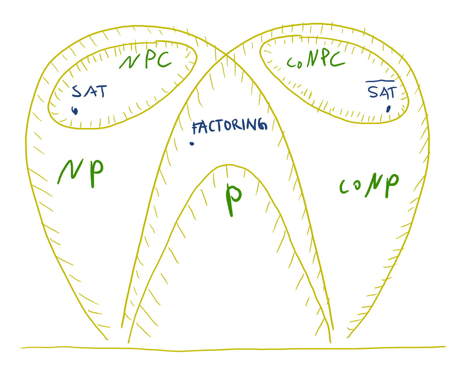
Conjectured landscape of NP vs coNP

The following sections give examples of problems with good characterizations. Some of these problems are also known to be in \({\mathrm{P}}\) (using more involved algorithms). Other problems, for instance \({\mathrm{FACTORING}}\), are not known to be in \({\mathrm{P}}\) (and conjectured to be intractable by some researchers).

Example: Systems of linear equations

LINEQ. Given a system of linear equations, decide if the system is satisfiable. (More formally, we are given a matrix \(A\in \mathbb Q^{m\times n}\) and a vector \(b\in \mathbb Q^{m}\) —with all numbers in binary representation— and the goal is to decide if there exists a vector \(x\in \mathbb Q^{n}\) such that \(A x = b\).)

We can solve this problem in polynomial-time by Gaussian elimination. It turns out that analyzing the running time of Gaussian elimination is quite subtle when taking into account bit complexity for arithmetic operations. ¹

We discuss how to show that LINEQ has a good characterization.

Theorem. \({\mathrm{LINEQ}}\in {\mathrm{NP}}\cap{\mathrm{coNP}}\).

First, we show that the problem is in NP.

Lemma. \({\mathrm{LINEQ}}\in {\mathrm{NP}}\).

Proof sketch. Given \(A\), \(b\), and \(x\), checking \(A x = b\) takes time polynomial in the bit complexity of \(A\), \(b\), and \(x\). (The fact that integer multiplication and addition take polynomial-time also implies that matrix-vector multiplication takes polynomial-time.) It remains to show that every satisfiable system of linear equations \(\{A x = b\}\) has a solution \(x\) with bit complexity polynomial in the bit complexity of \(A\) and \(b\). This fact can be shown by bounds on determinants. See homework 5, question 3 for more detailed hints. \(\qedhere\)

In order to show that \({\mathrm{LINEQ}}\in {\mathrm{coNP}}\), we will use the following linear algebra fact.

Linear algebra fact. For every system of linear equations \(\{ A x = b\}\) with \(A\in \mathbb Q^{m\times n}\) and \(b\in \mathbb Q^{m}\), either there exists \(x\in \mathbb Q^n\) with \(A x = b\) or there exists \(y\in \mathbb Q^m\) such that \(y^\top A = 0\) and \(y^\top b = 1\).

Note that \(y^\top A = 0\) and \(y^\top b=1\) implies that the system \(\{A x = b\}\) is not satisfiable, because every \(x\) satisfies \(y^\top (A x -b)= (y^\top A)x - y^\top b = 1\), which means that \(Ax - b \neq 0\). We give a geometric proof for this fact at the end of this section.

The above linear algebra fact implies the following reduction between LINEQ and its complement.

Lemma. \(\overline{\mathrm{LINEQ}}\le_p {\mathrm{LINEQ}}\).

Proof. Let \(A\in \mathbb Q^{m\times n}\) and \(b\in \mathbb Q^{m}\). By the above linear algebra fact, the linear system \(\{A x = b\}\) is not satisfiable if and only if the linear system \(\{ y^\top A = 0, y^\top b = 1\}\) is satisfiable. In matrix form, the latter system is \(\{ B y = c\}\), where \[ B= \left ( \begin{array}{c} A^\top\\ b^\top \end{array}\right) \quad\text{and}\quad c = \left ( \begin{array}{c} 0^n\\ 1 \end{array}\right ). \] It follows that the function mapping \((A,x)\) to \((B,c)\) as above is a polynomial-time Karp reduction from \(\overline {\mathrm{LINEQ}}\) to \({\mathrm{LINEQ}}\) \(\qedhere\)

Proof of theorem. The previous lemmas—\({\mathrm{LINEQ}}\in {\mathrm{NP}}\) and \(\overline {{\mathrm{LINEQ}}} \le_p {\mathrm{LINEQ}}\)—together imply \(\overline {\mathrm{LINEQ}}\in {\mathrm{NP}}\) (recall homework 3 question 2), which means that \({\mathrm{LINEQ}}\in {\mathrm{NP}}\cap {\mathrm{coNP}}\). \(\qedhere\)

Proof of linear algebra fact. Let \(A\in \mathbb Q^{m\times n}\) and \(b\in \mathbb Q^{m}\). We are to show that the system \(\{Ax = b\}\) has a solution if and only if the system \(\{y^\top A = 0, y^\top b = 1\}\) does not have a solution. Let \(U=\{A x \mid x \in \R^n\}\) be the linear subspace of \(\R^m\) spanned by the columns of \(A\). We decompose \(b\) as the sum \(b=c+y\) such that \(c\in U\) and \(y\) is orthogonal to \(U\). (Geometrically \(c\) is the point in \(U\) closest to \(b\) in Euclidean distance.) Since \(y\) is orthogonal to \(U\), it satisfies \(y^\top A = 0\) (which means geometrically that \(y\) is orthogonal to the columns of \(A\)). 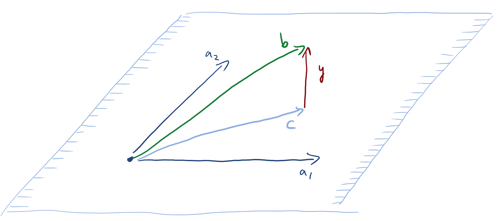By the construction of \(y\), the system \(\{Ax=b\}\) is satisfiable if and only if \(y=0\). Since \(b=y+c\), the vector \(y\) satisfies \[\lVert y \rVert_2^2 = y^\top y = y^\top (b-c)= y^\top b.\] It follows that \(y\neq 0\) if and only if \(y^\top b \neq 0\). Therefore, by scaling \(y\) appropriately, we obtain a solution for \(\{y^\top A = 0, y^\top b = 1\}\) if and only if \(\{A x=b\}\) is not satisfiable. \(\qedhere\)

Example: Maximum flow and minimum cut

In the following, a flow network is a directed graph with dedicated source and sink, and nonnegative integer capacities assigned to edges.

MAXFLOW. Given a flow network \(G\) and a number \(v\in \N\), decide if there exists a flow of value larger than \(v\) in \(G\).

The following problem turns out to be closely related (by the max-flow min-cut theorem below).

MINCUT. Given a flow network \(G\) and a number \(v\in \N\), decide if there exists a source-sink cut of capacity at most \(v\) in \(G\).

Both MAXFLOW and MINCUT are problems in \({\mathrm{P}}\) (using fairly sophisticated combinatorial algorithms). Below we will discuss how to show that these problems have good characterizations.

Theorem. \({\mathrm{MAXFLOW}}, {\mathrm{MINCUT}}\in {\mathrm{NP}}\cap {\mathrm{coNP}}\).

Recall that the Ford–Fulkerson algorithm shows the following interesting-trivial fact.

Fact. Every flow network (with integer capacities) has a flow of maximum value that the flow values along all edges are integers.

This fact allows us to conclude that \({\mathrm{MAXFLOW}}\in {\mathrm{NP}}\): Given a network \(G\), a number \(v\), and a potential flow \(f\), we can verify in polynomial time if \(f\) is a valid flow in \(G\) of value larger than \(v\). Furthermore, if there exists a flow of value larger than \(v\), then there is also one with bit complexity bounded by the bit complexity of \(G\). (Here, we use the fact above.) It is also straightforward to show that MINCUT is in NP.

Lemma. Both MAXFLOW and MINCUT are decision problems in NP.

Also recall that the analysis of the Ford–Fulkerson algorithm showed the following connection between MAXFLOW and MINCUT.

Maximum-flow minimum-cut theorem. For every flow network, the maximum value of a flow is equal to the minimum capacity of a source-sink cut.

Together with the previus lemma, the max-flow min-cut theorem allows us to show that MAXFLOW and MINCUT are also in coNP.

Lemma. \(\overline{\mathrm{MAXFLOW}}\le_p {\mathrm{MINCUT}}\) and \(\overline{\mathrm{MINCUT}}\le_p {\mathrm{MINCUT}}\).

Proof. In the problem \(\overline {\mathrm{MAXFLOW}}\), we are given a network \(G\) and a number \(v\) and we are to decide if the maximum flow in \(G\) is at most \(v\). By the max-flow min-cut theorem, this question is equivalent to the question whether \(G\) has a source-sink cut of capacity at most \(v\). It follows that \(\overline{\mathrm{MAXFLOW}}\le_p {\mathrm{MINCUT}}\). The argument for \(\overline{\mathrm{MINCUT}}\le_p {\mathrm{MINCUT}}\) is similar. (Note that we actually showed that \(\overline{\mathrm{MAXFLOW}}\) and \({\mathrm{MINCUT}}\) are the same problem in the sense \(\overline {\mathrm{MAXFLOW}}= {\mathrm{MINCUT}}\).) \(\qedhere\)

Example: Primality

Recall that a number is prime if it is greater than 1 and has no positive divisors other than 1 and itself. Here we consider the problem of testing if a given number is prime.

PRIMES. Given a number \(p\in \mathbb N\) encoded in binary, decide if \(p\) is prime.

For this problem a good characterization has been known since 1976 (Pratt).

Theorem. \({\mathrm{PRIMES}}\in {\mathrm{P}}\cap {\mathrm{coNP}}\).

Also polynomial-time randomized algorithms—by Miller–Rabin and Solovay–Strassen—have been known for this problem since around the same time. It has been an open problem to remove the use of randomness in these tests of primality. In 2002, Agrawal, Kayal, and Saxena showed that this problem indeed has a deterministic polynomial-time algorithm.

Theorem. \({\mathrm{PRIMES}}\in {\mathrm{P}}\)

Example: Integer factoring

The following problem plays a central role in cryptography (especially public-key encryption). An efficient algorithm for this problem could be used to break many cryptographic protocols used today, in particular RSA.

FACTORING. Given numbers \(x,a,b\in \mathbb N\) encoded in binary, decide if there exists a prime factor \(p\) in the interval \([a,b]\) such that \(p\) divides \(x\).

In order to give evidence for the security of current cryptographic protocols, it would be great to be able show that FACTORING is NP-complete. (Such a proof would not imply that the protocols are actually secure but it would still boost our confidence in their security.) However, it turns out that FACTORING has a good characterization, which means that it is not NP-complete unless NP is equal to coNP.

Theorem. \({\mathrm{FACTORING}}\in {\mathrm{NP}}\cap {\mathrm{coNP}}\).

Proof. The problem is in NP because the prime factor \(p\) is a polynomial-length certificate for YES instances: Using the polynomial-time algorithm for PRIMES, we can verify in polynomial-time that \(p\) is a prime. We can also verify \(p\in [a,b]\) and that \(p\) divides \(x\).

The problem is also in coNP because a prime factorization of \(x\) is a polynomial-length certificate for NO instances: Given numbers \(p_1,\ldots,p_k\), we can check that \(p_1,\ldots,p_k\) is a prime factorization of \(x\) (again using the polynomial-time algorithm for PRIMES) and that none of the primes \(p_1,\ldots,p_k\) are in the interval \([a,b]\). Here, we also use the fact that the prime factorization of a number is unique. \(\qedhere\)